Initialization Algorithm Description

The proposed initialization algorithm, called friends-and-enemies initialization, is designed to split the acoustic data to be processed into $K_{init}$ clusters, where $K_{init}$ is determined beforehand by the algorithm presented in 4.2.2 or manually set by the user. In the agglomerative clustering scheme presented for the meeting domain, it corresponds to the initial number of clusters used to start the agglomerative process. Each of the resulting initial clusters has a duration which is not restricted to be equal to any other cluster.

Figure 4.5: Clusters initialization blocks diagram

The complete initialization is composed of three distinct blocks, as shown in Figure 4.6. The first block performs a speaker-change detection on the acoustic data to identify segments with a high probability of containing only one acoustic event. Such acoustic events can either be silence, various noises, an individual speaker or various speakers overlapping each other. This first step is performed using the modified Bayesian Information Criterion (BIC) metric (introduced by Ajmera and Wooters (2003)) computed between two models created from the data in two adjacent windows of size $W$, connected at the evaluated possible change point. The modified $\Delta$BIC metric is computed over all the acoustic data every $S$ frames. A possible change point is selected if $BIC < 0$, it corresponds to a local minimum of the $\Delta$BIC values around it, and there is no other possible change point with smaller $\Delta$BIC value which is closer than $MD$ frames to it. In the implementation $W=2$ second windows are used, with a scroll $S = 0.5$ seconds. Each window is modeled using a model with 5 Gaussian mixtures (therefore with 10 Gaussians for the combined model) and a $MD$ of 3 seconds, equal to the minimum speaker turn duration used in the following agglomerative-clustering process.

The second block in the initialization algorithm creates clusters by identifying the segments defined in the first part as friends or enemies of each other. It is considered that two given acoustic segments are friends if they contain acoustically homogeneous data; only the best friends are brought together to form a cluster. In the same way, it is considered that two segments are enemies if they contain very dissimilar acoustic data. It is intended to obtain $N$ final enemy groups (the desired final number of clusters) consisting of $F$ segments each, which are friends of each other. Three different similarity metrics were experimented with to compare each segment pair $S_{1}$ and $S_{2}$. On the first place a geometric mean of the frame cross-likelihood as

$$d_{1}(S_{1}, S_{2}) = \frac{\log \mathcal{L}(S_{1}\vert\Theta_{S_{2}}) + \log \mathcal{L}(S_{2}\vert\Theta_{S_{1}})}{(N_{S_{1}} + N_{S_{2}})}$$ (4.6)

where $N_{S_{i}}$ is the number of frames in segment $i$, and $\Theta_{S_{i}}$ is a model with 5 Gaussian Mixtures trained with $S_{i}$.

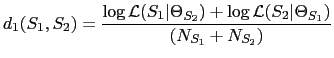
The second metric normalizes each term by the number of frames in the linear domain instead, resulting in a penalty to the cross-likelihood as

$$d_{2}(S_{1}, S_{2}) = \log lkld(S_{1}\vert\Theta_{S_{2}}) + \log lkld(S_{2}\vert\Theta_{S_{1}}) - \log L_{S_{1}} - \log L_{S_{2}}$$ (4.7)

The third metric does a full cross-likelihood as introduced by Rabiner in Juang and Rabiner (1985)

$$d_{3}(S_{1}, S_{2}) = \log lkld(S_{1}\vert\Theta_{S_{2}}) + \log... ...}) - \log lkld(S_{1}\vert\Theta_{S_{1}}) - \log lkld(S_{2}\vert\Theta_{S_{2}})$$ (4.8)

All three metrics are bigger the closest the segments are to each other. In order to initiate the process one needs to define an initial segment. Again, three criteria have been considered:

1. Select the segment which is most representative of the meeting, which might indicate that it belongs to the speaker with most participation. In order to find it, a global GMM with 16 Gaussian mixtures is trained using all data in the meeting and the segment with biggest likelihood (normalized using geometric mean) is chosen.

2. Select the segment which is the least representative of the meeting, which might indicate that it belongs to the speaker with smallest participation. Using the same GMM model as before, the segment with smallest averaged likelihood is chosen.

3. Select the segment with the closest average distance to all other segments. Using one of the distances presented above, the average of distances between each segment and all other segments is computed and the maximum is chosen.

Figure 4.6: Friends-and-enemies clusters initialization process

Figure 4.6 shows an example case on how the algorithm works. In the horizontal axis the speaker segments as found by the first block, are represented. The vertical axis shows the distance value associated to each segment. In step (0) the initial segment needs to be determined. In this example the criterion 2 is used to find the segment with smallest averaged likelihood, $S_{1}$.

Then, in step (1a) the data in $S_{1}$ is used to train a model with 5 Gaussian mixtures ( $\Theta_{S1}$) and compute either metric $d_{1 \cdots 3}$ between itself and all other segments. The $F-1$ segments with bigger value are its friends. In this example, $F=3$ and the selected friends for $S_{1}$ are chosen to be $S_{5}$ and $S_{7}$. In step (1b), a new model is trained from all data in this first cluster ( $\Theta_{1}$) and the same metric as before is computed, except that now it is measured between all segments in the model and each of the remaining segments.

A new enemy $S_{2}$ is selected as the segment with smaller value to the first cluster. Also in the same way, in step (2a) $F-1$ friends are chosen for $S_{2}$ and in (2b) we select a new enemy for both previously established clusters. This is done by computing the sum of the used metric for each segment given all predefined groups. The processing continues until the desired number of initial clustering $N$ is reached or it runs out of free segments.

At that point in the third block all created models are used to reassign the acoustic data into the $K_{init}$ classes. This is done using a Viterbi decoding where the resulting segmentation is not constrained to the predefined speaker changes, therefore any previous speaker change detection errors can be corrected. All data gets assigned to its closest cluster, classifying any acoustic frames not assigned in the previous block. Finally, one cluster model is trained from each of the resulting clusters.