Models Training Using CV-EM and Clusters Segmentation

In order to train the speaker models used throughout the processing a standard EM-ML algorithm was used by the broadcast news system. It performed a five iterations EM-ML algorithm regardless of the data or the models being trained. The use of EM in small training datasets has two potential problems. On one hand the models can suffer from overfitting to the available data, becoming not general enough to represent the speaker at hand. On the other hand there is no guarantee that the models will converge to the best possible parameters that maximize the likelihood of the data given such model. The use of $k=5$ iteration of EM training is a parameter that needs to be defined for the system in order to avoid overfitting but to allow the models to be correctly trained to the data. It was seen that modifying the value of the parameter $k$ would considerably alter the final performance, and therefore it was found desirable to find a more robust algorithm.

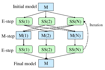
For these reasons a new training algorithm has been implemented. The choice of implementation has been the cross-validation EM training algorithm (CV-EM for short), recently proposed by T. Shinozaki in Shinozaki and Ostendorf (2007). It introduces a cross-validation technique, in use for decision tree design, to the iterative process of the EM, addressing the problems of overfitting and potential local maxima.

Figure 3.8: Cross-validation EM training algorithm

Figure 3.8 shows the CV-EM procedure. The system starts from an initial single model to be trained and finishes also with a single model. On the initial E-step of the EM processing the training data is split into N partitions as homogeneously as possible (in the implementation each consecutive frame is assigned to a different partition sequentially until all frames have been assigned). Then the conditional probability of each frame to each Gaussian mixture in the initial model is computed. This process is identical to the initial E-step in a similar technique called parallel EM training (Young et al., 2005).

In the following M-step, each model $M_{i}$ is reestimated using the sufficient statistics computed for all partitions except for $SS_{i}$, which is kept as cross-validation data. This differs from the parallel EM technique, which collapses all the statistics into creating a single model, losing the cross-validation properties. In the CV-EM algorithm, once all the N models have been approximated, new conditional probabilities are computed for the frames in each partition $SS_{i}$ using model $M_{i}$. As data in partition $SS_{i}$ has not been involved in the reestimation of the parameters in $M_{i}$, the accumulated likelihood from all partitions can be used as a cross-validation to check for convergence, avoiding the possible overfitting to the data. In the implementation a $\Delta \mathcal{L}_{inc} = 0.1$% likelihood increase criterion is used.

In Shinozaki and Ostendorf (2007) it proposes a 5 iterations step when training models towards speech recognition, although in speaker diarization a likelihood relative increase stopping criterion is preferred in order to bound the likelihood variation between iterations.

Given two clusters $A$ and $B$, with data $X_{A}$ and $X_{B}$ and their respective models, $M_{A}$ and $M_{B}$, when training such models let us consider the variation in likelihood between two EM iterations as $\Delta \mathcal{L}(X_{A}\vert M_{A})$ and $\Delta \mathcal{L}(X_{B}\vert M_{B})$. Within the diarization system we want to use the $\Delta$BIC metric to determine wether they belong to the same speaker or not. By using the modified $\Delta$BIC constrained by 3.2, and expanding terms, we obtain:

$$\Delta BIC(A,B) = \log \mathcal{L}(X_{A}\vert M_{A+B}) + \log \mathcal{L}(X_{B}\vert M_{A+B})$$

$$- \log \mathcal{L}(X_{A}\vert M_{A}) - \log \mathcal{L}(X_{B}\vert M_{B})$$ (3.3)

In the usual proceeding of the algorithm, by comparing the resulting $\Delta$BIC value to a threshold 0 it will be determined wether both clusters are the same speaker or not. If each of the models is trained an extra EM iteration, and using the notation introduced before, one can express the resulting $\Delta^{'}$BIC in terms of the one just computed in equation 3.3 as

$$\Delta BIC'(A,B) = \Delta BIC(A,B) + \Delta \mathcal{L}(X_{A}\vert M_{A+B}) + \Delta \mathcal{L}(X_{B}\vert M_{A+B})$$

$$- \Delta \mathcal{L}(X_{A}\vert M_{A}) - \Delta \mathcal{L}(X_{B}\vert M_{B})$$ (3.4)

In order for the system to be robust and results consistent it is desired that $BIC'(A,B) = BIC(A,B)$ which leads to having the likelihood variation terms to cancel out. While it is not possible to control the exact likelihood variations between iterations, by using a minimum relative likelihood variation as a stopping criterion for the CV-EM training makes these terms upper bounded and the BIC more stable. Furthermore, by forcing these variations to be small will result in $BIC(A,B) \simeq BIC'(A,B)$ as desired.

According to Shinozaki and Ostendorf (2007), since N cross-validation models are reestimated from different subsets of the data it could potentially create a problem where the Gaussian mixtures would behave differently to the data and obtain totally different parallel models, in which case the CV-EM algorithm would not be usable. In reality the difference in number of samples between any two models is $\frac{1}{N-1}$, which becomes very small when N is large, and therefore prevents this divergence from happening.

Once the CV-training stopping criterion is reached, the current sufficient statistics computed for each of the subsets are used to derive a single output model. The increase in computation for this parallel training technique is small as only in the M-step the number of operations is increased. When the size of the training data is big, the most costly part of the EM algorithm is the E-step, which takes the same time to be computed as by the CV-EM algorithm.

In order to avoid quick changes in the speaker turns in both the baseline and the current system, a minimum duration of 3 seconds is imposed when performing Viterbi segmentation of the data. This is imposed in the speaker model by using multiple consecutive states with transition probability 1 between them, and tied Gaussian mixture models, as seen in figure 3.2.

On the contrary, it was observed that the maximum turn duration for the speaker turn is artificially constrained by the $\alpha$ and $\beta$ parameters in figure 3.2. As explained in detail in section 4.2.3 these were changed to $\alpha=1$ and $\beta=1$ to allow the maximum duration to be solely decided by the acoustics. This is an important change given that conference room data is very different in terms of average speaker turn length to broadcast news and to lecture room data.

As mentioned earlier, when processing multiple microphones the system creates an independent feature stream to the acoustic stream composed of the TDOA values between microphones. As explained in section 5.3, each one of the feature streams is represented by different models and the total likelihood of the data at any instant is obtained as the weighted sum of the log-likelihood of the respective feature vectors according to their models. The resulting log-likelihood affects the decisions made in the Viterbi segmentation module and in the $\Delta$BIC computation between two clusters, which otherwise are identical to the broadcast news system.

In order for the different independent feature streams to be combined at the log-likelihood level a relative weight has to be assigned for each one depending on their reliability to contribute to the diarization. Although an initial weight is set for all meetings using development data, each particular meeting will respond differently to the use of the TDOA values and therefore an automatic system of reestimating these initial weights is desirable. An effective way was found using a metric derived from the $\Delta$BIC values computed between all pairs for all feature streams. It is described in section 5.3.2.