Next: Rich Transcription evaluation datasets Up: Robust Speaker Diarization for Previous: Possible Future Work Topics Contents
The purpose of this appendix is to show the equivalence between two different representations of the Bayesian Information Criterion (BIC), one based on the likelihood of the data given the models, which allows the models to be arbitrary and as complex as necessary given the task at hand, and another representation only dependent on the sufficient statistics of the data, which considers the case of a single Gaussian modeling the data. These two representations are used alternatively in the bibliography with various modifications, which sometimes cause the results not to be comparable between each other.
Given an acoustic segment ![]() with
with ![]() acoustic frames,
modeled by
acoustic frames,
modeled by ![]() which is an arbitrary model with a certain
number of free parameters to estimate from the data, given by
which is an arbitrary model with a certain
number of free parameters to estimate from the data, given by
![]() , which accounts for the complexity of such
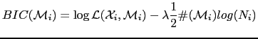
model. The general BIC expression of such model using the
likelihood of the data is given by
, which accounts for the complexity of such
model. The general BIC expression of such model using the
likelihood of the data is given by
Being
![]() the log-likelihood of the data given the considered model. The
parameter
the log-likelihood of the data given the considered model. The
parameter ![]() is a design parameter which is not part of the
original BIC formulation but which is used to change the effect of
the penalty term in the formula. Such formula allows the model
is a design parameter which is not part of the
original BIC formulation but which is used to change the effect of
the penalty term in the formula. Such formula allows the model
![]() to be of any kind.
to be of any kind.
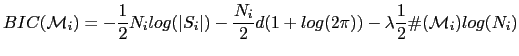
If instead it is considered that the model is created by a single Gaussian, eq. A.1 can be rewritten as
where ![]() is the covariance matrix representing the data
and
is the covariance matrix representing the data
and ![]() is its dimension. Such formulation only depends on the
sufficient statistics of the data, and therefore its computation
is very fast.
is its dimension. Such formulation only depends on the
sufficient statistics of the data, and therefore its computation
is very fast.
Let us progress from equation 2.1 into obtaining equation A.2. Considering that the used model is a single Gaussian with full covariance, one can rewrite eq. 2.1 as
by doing the ![]() products one obtains a sum of terms
in the exponential, where each terms is a scalar value. One can
use mathematical properties of the trace in order to obtain a
closer form for it. As the trace(scalar) = scalar, it does not
change the result.
products one obtains a sum of terms
in the exponential, where each terms is a scalar value. One can
use mathematical properties of the trace in order to obtain a
closer form for it. As the trace(scalar) = scalar, it does not
change the result.
Let us then consider only the trace of the numerator in the exponent
Given this result and going back to the BIC formulation in eq. A.3 and using the log properties
![$\displaystyle BIC(\mathcal{M}_{i}) = \log [\frac{1}{(2\pi)^{dN_{i}/2}\vert S\vert^{N/2}} e^{-N_{i}d/2}] $](img533.png)
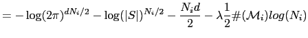
Obtaining finally
 |
(A.4) |
Which is in fact equation A.2. Note that a factor
![]() applies to each term in the expression. Such factor
is sometimes omitted, causing the optimum
applies to each term in the expression. Such factor
is sometimes omitted, causing the optimum ![]() factor to
differ in the different implementations.
factor to
differ in the different implementations.
![$\displaystyle BIC(\mathcal{M}_{i}) = \sum_{n=1}^{N_{i}} \log p(x_{i}[n]\vert\m...
...\vert^{1/2}} \exp^{-\frac{1}{2}(x_{i}[n]-\bar{x})' S^{-1} (x_{i}[n]-\bar{x})}]$](img527.png)